Excel: Identify Duplicates

While the previous post in this series described how to remove duplicate values in Excel, this post describes how to identify duplicates.

The remove duplicates function doesn’t tell you which values are duplicates, it just removes them. Sometimes you need a list of the duplicates so you can review them in detail or include them in your workpapers.

So we’ll look at how to create a list of duplicates across all values/columns and in specific columns.

These procedures are written for Excel 2013, but the same steps should also work in Excel 2010, but the screenshots might be a little different.

Identifying Duplicates Across All Columns

To identify duplicates across all values (columns) in an Excel table:

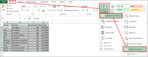
1. Highlight all the cells that you want to analyze.
   In Example 1 below, I selected all cells in the table (to enlarge an example, click it). To highlight the table, click in cell A1, and while holding the mouse button, drag down to cell D11. Release the mouse button.
   
2. On the Home tab, click the following: Conditional Formatting, Highlight Cell Rules, Duplicate Values.
   See Example 1 below.
   
   

   Example 1

   
   

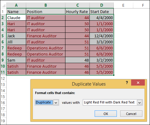
3. The Duplicate Values dialog box appears, and the duplicates in each column are highlighted immediately. Accept the default values, and press OK.
   See Example 2 below.
   
   

   Example 2

   
   

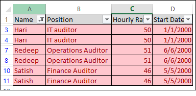
4. Notice the following in Example 2 above:
   – In column A, Hari, Redeep, and Satish are the only duplicate names (red). Claude, Jack, Jill, and Sam (grey) are unique values.
   – In column B, all the values are red, and no unique values exist.
   – In column C, the only unique value is 48 (grey)
   – In column D, 4 dates are unique (grey) and the rest are duplicates (red).
5. To list the rows that contain duplicate values across all columns, you have to filter the values. This is a 3-step process.
   First, position the cursor in row 1; when the cursor changes to an arrow, click once to highlight the entire row.
   See Example 3 below.
   
   

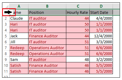
   Example 3

6. Second, apply the filter arrows to the columns: in the Data tab, click Filter.
   See Example 4 below (the filter arrows don’t appear until after this step–see Example 5  further down).
   

   Example 4

7. Third, in column A, click the filter arrow, Filter by Color, and then the light red color (which identifies duplicate values) under Filter by Cell Color.
   See Example 5 below.
   
   

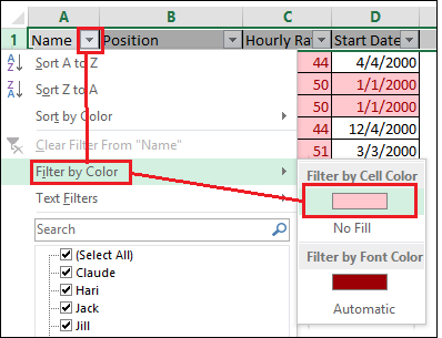
   Example 5

8. The result is a list of duplicates across all columns.
   This is the list that you can save in your workpaper.
   See Example 6 below.
   
   

   Example 6

One Important Note

Because of how this Excel function works, be careful if any cell in one column contains data that is identical to the data in another column.

For example, assume we have a table similar to Example 3 in step 5 above, except that it contains “Jill” in cell B9 (which is identical to the value in cell A6). When you analyze this table, ‘Jill’ will be flagged as a duplicate in both places. See red boxes in Example 3a below.

Example 3a

When you filter this table for duplicates across all cells, you get the result shown below in Example 3b below. The fact that cell D6 (3/3/2000) is white tells you something is not right.

Example 3b

However, by looking at the original data (Example 3a above), it’s clear that the two rows containing Jill are NOT duplicates of each other. Therefore, row 6 can be safely filtered out (in column D, use the filter to deselect 3/3/2000 so that the entire row is hidden).

The result is a correct listing of duplicates across all columns, shown in Example 3c below.

Example 3c

Keep in mind that this example is a little obvious, as values like ‘Jill’ would not normally appear in a column named Position.

However, if you have a table that contains columns called First Name and Last Name, that could be more of a challenge. If ‘Simon’ was one person’s first name and another person’s last name (which is not uncommon in the USA), you’d have the same condition, and that would be easier to miss when you analyze for duplicates.

I don’t think this issue will occur very often, and when it does, you can catch it by noticing values that are not shaded light red. So in conclusion, I still think using this Excel function to identify duplicates is a good one.

But be careful out there, and always check your results.

A shout-out to John, who raised this question in the comments. Thanks!

See all the posts for these series at Excel: Basic Data Analytic series.